This post explains the roofline model with measurements from six NVIDIA GPUs and two AMD GPUs; all numbers, figures and code are in the companion repository. The main conclusions:
- If a GPU program does more operations per byte moved (FLOP/byte) than the hardware’s ridge point (compute divided by bandwidth, also in FLOP/byte), compute limits it; otherwise bandwidth does.
- On one GPU, each precision and each compute unit has its own peak compute and thus its own ridge point: on H100, 255 FLOP/byte for FP16 Tensor Core and 19.9 FLOP/byte for FP32 CUDA Core.
- In the FP16/BF16 linear layers of a large language model, this ratio is about the number of tokens fed in at once. The model first feeds in all input tokens together (prefill), limited by compute when the input is long; then each step feeds in the 1 token the previous step generated (decode), limited by bandwidth.
- Each decode step reads all the weights once, so bandwidth sets its speed. Requests computed together share this read, so the more requests computed together, the faster each token on average.
Highlights in the text: core concept conclusion how to judge practical use
1. Two lower bounds on time
The roofline model answers two questions: how fast a GPU program can run at most on a given GPU, and whether moving data or doing arithmetic limits it.
A GPU program is made of kernels. A kernel is a function that runs in parallel on the GPU; the CPU issues it, and each issue is a launch. While a kernel runs, the hardware moves data between GPU memory and the chip and does arithmetic in its compute units. Four quantities describe both:
| Doing arithmetic | Moving data | |
|---|---|---|
| Work of the kernel | \(W\): operations (FLOP) | \(Q\): GPU memory traffic (byte) |
| Hardware limit per second | \(F\): peak compute (FLOP/s) | \(B\): memory bandwidth (byte/s) |
Table 1: The four quantities of the roofline model. One floating-point add or multiply counts as 1 FLOP.
\(W\) operations take at least \(W/F\) seconds, and moving \(Q\) bytes takes at least \(Q/B\) seconds. A kernel ends when both are done, so its run time is
\[T \ge \max\!\left(\frac{W}{F},\ \frac{Q}{B}\right)\]Arithmetic and data movement use different parts of the chip and can overlap, so the real time can approach the larger of the two.
Comparing the two terms is equivalent to comparing two ratios:
\[\frac{W}{F} > \frac{Q}{B} \iff \frac{W}{Q} > \frac{F}{B}\]\(W/Q\) depends only on the kernel and \(F/B\) only on the hardware; the next two sections cover each. The whole model is a comparison of these two ratios.
2. Arithmetic intensity
Arithmetic intensity \(I = W/Q\) is the number of operations a kernel does for each byte it moves, in FLOP/byte. It depends only on the shape and precision of the operation and can be computed directly from the formula.
Matrix multiply. In a matrix multiply (often written GEMM) \(X_{M\times K} \cdot A_{K\times N} = Y_{M\times N}\), \(Y\) has \(MN\) elements, each taking \(K\) multiplies and \(K\) adds, so \(W = 2MNK\). \(Q\) counts each matrix read or written once: \(MK + KN + MN\) elements.
Write sizeof for the bytes per element: 8 for FP64 (double), 4 for FP32 (float), and 2 for the two half-precision formats FP16 and BF16. Then
\[I = \frac{2MNK}{\text{sizeof} \cdot (MK + KN + MN)}\]Four common operations. The element-wise operation \(y = x \cdot a + b\) (\(x\), \(y\) arrays; \(a\), \(b\) constants) reads and writes each element once and does 1 FMA (fused multiply-add: one instruction for a multiply and an add, counted as 2 FLOP), so \(I = 1/\text{sizeof}\). The other three simplify the formula above for different matrix shapes. A thin matrix has \(M\) much smaller than \(N\) and \(K\), so the denominator is about \(\text{sizeof} \cdot KN\).
| Operation | \(I\) (FLOP/byte) | FP32 | FP16 |
|---|---|---|---|
| Element-wise \(y = x \cdot a + b\) | \(1/\text{sizeof}\) | 0.25 | 0.5 |
| Square matrix \(M = N = K = n\) | \(2n / (3 \cdot \text{sizeof})\) | \(n/6\) | \(n/3\) |
| Thin matrix \(M \ll N = K\) | \(2M / \text{sizeof}\) | \(M/2\) | \(M\) |
| Matrix-vector multiply (GEMV) \(M = 1\) | \(2 / \text{sizeof}\) | 0.5 | 1 |
Table 2: Arithmetic intensity of the four operations, in FLOP/byte.
Table 2 shows two things:
- Precision changes \(I\). sizeof is in the denominator: moving the same matrix multiply from FP32 to FP16 halves \(Q\) and doubles \(I\).
- The shape sets the order of magnitude of \(I\). It is below 1 for element-wise operations, proportional to \(n\) for square matrices, and to \(M\) for thin ones.
LLM linear layers are thin matrices. A large language model (LLM) processes text as tokens (words or word parts), with most arithmetic in the linear layers \(Y = XA\). \(X\) holds \(M\) tokens as length-\(K\) vectors; \(A\) is a trained \(K \times N\) weight. With few tokens, \(M \ll K, N\), so an FP16/BF16 linear layer’s arithmetic intensity is about the number of tokens fed in at once. As \(M\) nears \(K\) and \(N\) in scale, \(I\) grows more slowly.
3. Roofline and ridge point
Throughput \(P = W/T\) is the number of operations a kernel completes per second (FLOP/s). Substituting the lower bound on \(T\):
\[P = \frac{W}{T} \le \frac{W}{\max(W/F,\ Q/B)} = \min(B \cdot I,\ F)\]For a given GPU, \(F\) and \(B\) are constants, and the bound varies only with \(I\). As a function of \(I\), it is a line that rises and then turns flat, shaped like a roof, hence the name roofline:
- Slope: for small \(I\), the bound is \(B \cdot I\) and bandwidth sets the time (memory-bound);
- Flat part: for large \(I\), the bound is \(F\) and compute sets the time (compute-bound);
- ridge point: the two parts meet at \(I^* = F/B\), the hardware ratio from Section 1. A kernel with \(I\) below \(I^*\) is memory-bound; above \(I^*\), compute-bound.
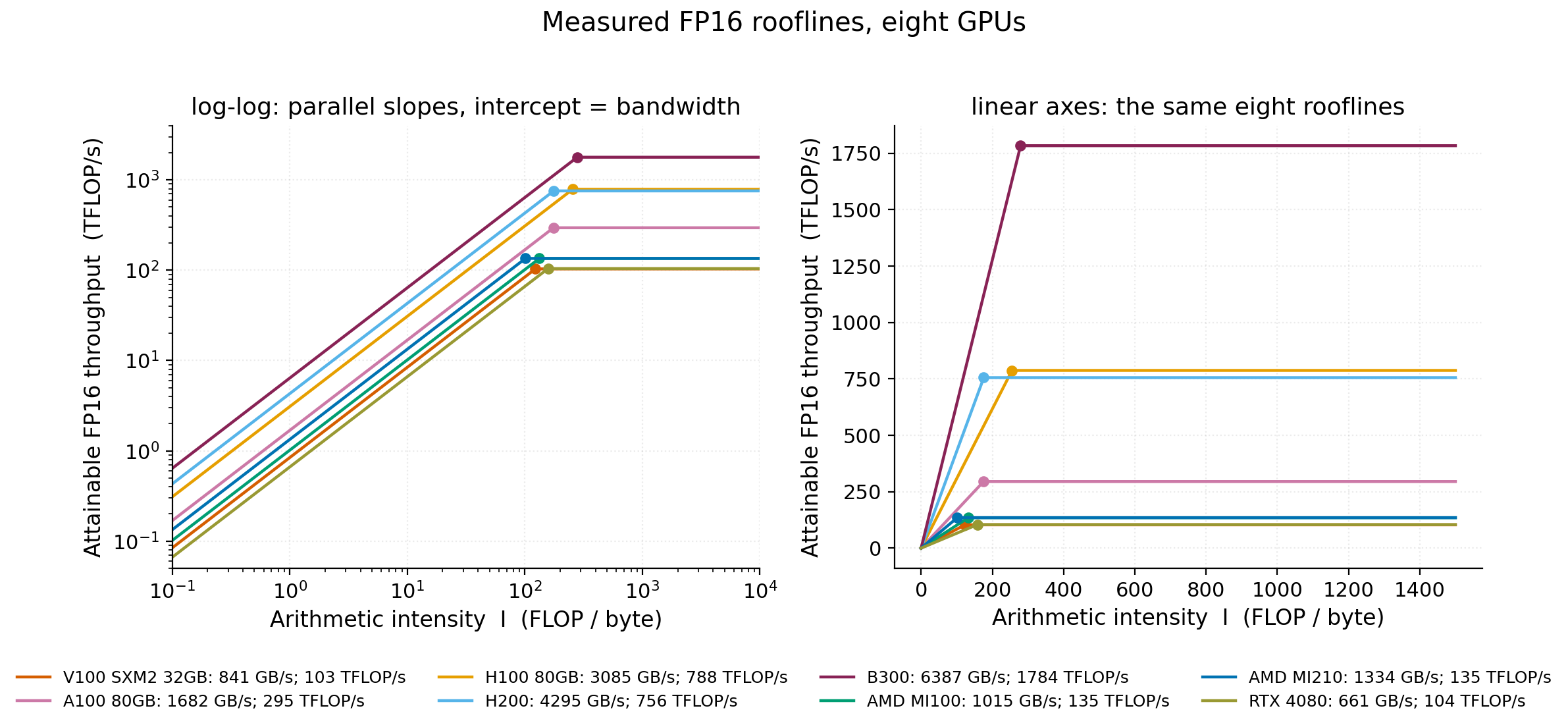
\(I\) spans several orders of magnitude, from a few tenths to over a thousand, so rooflines are usually drawn on log-log axes. There the slope is the line \(\log P = \log I + \log B\) with gradient 1; bandwidth changes only the intercept, so all GPUs’ slopes are parallel.
Rooflines of the eight GPUs
Figure 1 and Table 3 show the measured FP16 rooflines of eight GPUs. The first five are NVIDIA data-center GPUs, ordered by release from V100 (2017) to B300 (2025); MI100 (2020) and MI210 (2022) are AMD data-center GPUs; the RTX 4080 is a consumer gaming card.
| GPU | \(B\) GB/s | \(F\) FP16 TFLOP/s | \(I^*\) FLOP/byte |
|---|---|---|---|
| V100 SXM2 32GB | 841 | 103 | 123 |
| A100 80GB | 1682 | 295 | 176 |
| H100 80GB | 3085 | 788 | 255 |
| H200 | 4295 | 756 | 176 |
| B300 | 6387 | 1784 | 279 |
| AMD MI100 | 1015 | 135 | 133 |
| AMD MI210 | 1334 | 135 | 101 |
| RTX 4080 | 661 | 104 | 158 |
Table 3: Measured bandwidth, FP16 compute and ridge point of the eight GPUs. With \(F\) in TFLOP/s and \(B\) in GB/s, \(I^* = 1000 \times F / B\) (from unrounded values).
- Compute grew faster than bandwidth. From V100 to B300, \(F\) grew 17 times and \(B\) 7.6 times, and \(I^*\) moved right. The same kernel is more likely to be memory-bound on a newer GPU.
- The rooflines of H200 and H100 cross. H200 has 39% more bandwidth and slightly less compute (756 vs 788 TFLOP/s), and the rooflines cross at \(I = 245\) FLOP/byte: below it H200’s is higher, above it H100’s is slightly higher. Which GPU gives a kernel the higher bound depends on which side of the crossing its \(I\) falls.
- With equal \(F\), a larger \(B\) gives a smaller \(I^*\). AMD’s MI100 and MI210 both have 135 TFLOP/s of FP16 compute; MI210 has 31% more bandwidth (1334 vs 1015 GB/s), and \(I^*\) falls from 133 to 101 FLOP/byte.
- RTX 4080 is more likely to be memory-bound. Its \(F\) almost equals V100’s and its \(B\) is 79% of V100’s, so its \(I^*\) is larger (158 vs 123 FLOP/byte).
Multiple rooflines on one GPU
On one GPU, each precision and each compute unit has its own \(F\) and its own roofline.
A Tensor Core is a unit for small matrix multiplies, with far more compute than the CUDA Cores (ordinary arithmetic units) that run FMA instructions. Matrix multiplies can use Tensor Cores; element-wise operations, normalization (LayerNorm), softmax and other non-matrix-multiply operations common in LLMs can use only CUDA Cores.
TF32 is a mode in which Tensor Cores run FP32 matrix multiplies with a shorter mantissa. It is slightly less precise and usually off by default, so a default FP32 matrix multiply matches the “TF32 off” row of Table 4.
| Compute path on H100 | \(F\) TFLOP/s | \(I^*\) FLOP/byte |
|---|---|---|
| FP16 matrix multiply, Tensor Core | 788 | 255 |
| TF32 matrix multiply, Tensor Core | 418 | 135 |
| FP64 matrix multiply, Tensor Core | 64.2 | 20.8 |
| FP32 FMA, CUDA Core | 61.5 | 19.9 |
| FP32 matrix multiply, CUDA Core (TF32 off) | 51.9 | 16.8 |
| FP64 FMA, CUDA Core | 32.9 | 10.7 |
Table 4: Measured compute and ridge point of six compute paths on H100. Section 4 explains how the two FMA rows are measured.
- Judge by the path the kernel uses. Analyze a kernel with the roofline of the compute path it actually uses. A kernel with \(I = 50\) FLOP/byte is memory-bound on FP16 Tensor Cores (\(I^* = 255\)) and compute-bound on FP32 CUDA Cores (\(I^* = 19.9\)). FP32 LayerNorm and softmax run on CUDA Cores, where \(I^*\) is 19.9.
- FP64 matrix multiply is faster than FP32. On H100, FP64 matrix multiplies can use Tensor Cores (64.2 TFLOP/s); FP32 ones with TF32 off, CUDA Cores only (51.9). That is below FP32 FMA (61.5), since a matrix multiply kernel also runs load, store and synchronization instructions. If slightly lower precision is acceptable, TF32 puts FP32 matrix multiplies on Tensor Cores: 51.9 → 418 TFLOP/s.
- B300 has the largest gaps between paths. Its FP16 Tensor Core compute is 1784 TFLOP/s and its FP64 matrix multiply 1.05 TFLOP/s. Designed for low-precision AI computing, B300 has very few FP64 units; its FP64 \(I^*\) is 0.16 FLOP/byte, and almost every FP64 kernel is compute-bound on it.
4. Measuring bandwidth and peak compute
All \(F\) and \(B\) values in this post’s rooflines are measured on each GPU. The subsections below cover bandwidth and compute.
Bandwidth
Bandwidth is measured with kernels that only move data and do almost no arithmetic, such as one that reads a 512 MiB array and sums it.
Besides GPU memory, the GPU has a small, high-bandwidth on-chip L2 cache (A100 40 MiB, H100 50 MiB, RTX 4080 64 MiB). Measurements repeat the kernel many times; if all the data it reads and writes (the working set) fits in L2, later runs find it still there, giving L2 bandwidth. So measuring GPU memory bandwidth needs a working set much larger than L2. Figure 2 shows copy-kernel bandwidth by working set.
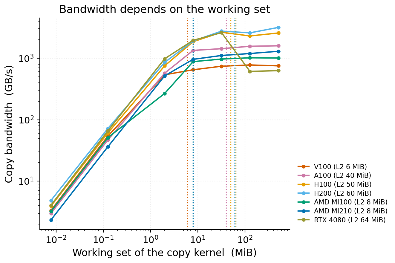
- Past the L2 size, the result is GPU memory bandwidth. RTX 4080’s 2600 GB/s at 32 MiB is L2 bandwidth; its 610 GB/s at 128 MiB is GPU memory bandwidth. On the other GPUs bandwidth changes little past L2: A100, H100 and H200 have memory bandwidth close to their L2 bandwidth, and V100, MI100 and MI210 have 6 to 8 MiB of L2, where launch overhead dominates the time.
- With a very small working set, the time is launch overhead. From a few KiB to a few MiB, bandwidth rises in proportion to working set. Each launch has a fixed cost of a few microseconds (launch overhead), almost all the time in this range: data doubles, time stays the same, and the computed bandwidth doubles.
Kernels written differently measure different bandwidths: on H100, the read-only kernel that sums 512 MiB measures 3085 GB/s and the copy kernel 2568 GB/s. The roofline’s \(B\) is the highest value among all kernels that only move data.
Compute
cuBLAS (NVIDIA’s matrix multiply library) runs two sets of matrix multiplies:
- square matrices, with \(n\) from 256 to 8192;
- thin matrices, with \(N = K = 8192\) fixed and \(M\) doubling from 1 to 2048, plus a final \(M = 8192\); this set is called the M sweep below.
\(F\) is the highest throughput over all shapes: 788 TFLOP/s for H100 FP16.
Measuring the shape of the roofline directly
The \(B\) and \(F\) above come from different kernels. One kernel can also sweep the whole x-axis, to test whether its throughput follows \(\min(B \cdot I,\ F)\).
The method modifies Section 2’s element-wise operation: each element, once read, goes through \(R\) consecutive FMAs in registers before being written back (called the FMA sweep below). Each element takes \(2R\) FLOP and is still read and written once, so
\[I = \frac{2R}{2 \cdot \text{sizeof}},\qquad \text{FP32: } I = R/4,\quad \text{FP64: } I = R/8\]\(R\) runs from 1 to 2048, and the arrays read and written total 512 MiB, much larger than L2.
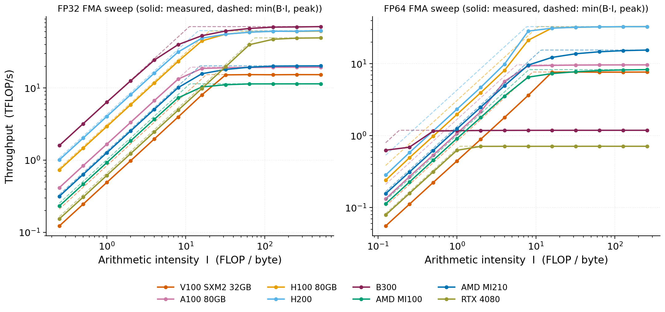
- Slope: the time is about that of moving 512 MiB; doubling \(R\) doubles the work, keeps the time, and doubles throughput.
- Flat part: the compute units are fully loaded; doubling \(R\) doubles the time too, and throughput stays constant.
- Rounded corner near the ridge point: measured values fall below the dashed line, because data movement and arithmetic cannot fully overlap.
- Some slopes sit lower: for V100 in FP32 and FP64, and for A100, H100 and H200 in FP64, this kernel uses 53% to 66% of memory bandwidth; elsewhere it mostly uses 88% or more. This comes from how the kernel is written and does not affect the height of the flat part.
The height of the FMA sweep’s flat part is the \(F\) of the ordinary arithmetic units (CUDA Cores on NVIDIA GPUs):
| GPU | FP32 FMA TFLOP/s | FP64 FMA TFLOP/s |
|---|---|---|
| V100 SXM2 32GB | 15.3 | 7.7 |
| A100 | 19.4 | 9.7 |
| H100 | 61.5 | 32.9 |
| H200 | 62.2 | 32.9 |
| B300 | 70.8 | 1.19 |
| AMD MI100 | 11.4 | 8.3 |
| AMD MI210 | 20.3 | 15.5 |
| RTX 4080 | 49.4 | 0.71 |
Table 5: Measured compute of the ordinary arithmetic units on eight GPUs.
- Consumer GPUs are short on Tensor Cores. RTX 4080’s FP32 FMA is 2.5 times A100’s, while its FP16 Tensor Core compute is 35% of A100’s.
- The FP64-to-FP32 ratio differs. On V100, A100, H100 and H200, FP64 is about half of FP32; on MI100 and MI210 it is 73% and 77%; B300 and RTX 4080 have few FP64 units and reach about 1 TFLOP/s in FP64.
5. Measured points and the roofline
Given a roofline, a kernel is a point on the plot: its x-coordinate is its \(I\), and its y-coordinate its measured throughput \(W/T\). The point shows two things:
- The part above the point sets what to optimize. Under the slope, the time bound is \(Q/B\), set by bytes moved alone; under the flat part, it is \(W/F\), set by work and compute alone. So under the slope, cut bytes moved and raise \(I\); under the flat part, move to a higher flat part, such as Tensor Cores or lower precision.
- Distance to the roofline shows the room left. The point’s y-coordinate over the roofline height at that x is the fraction of the bound reached. A kernel on the roofline has nothing left to optimize in its implementation: on the slope, only a higher \(I\) makes it faster; on the flat part, only a higher flat part.
Measured points of matrix multiply
Figure 4 places measured cuBLAS matrix multiply points under the rooflines of three GPUs in three precisions.
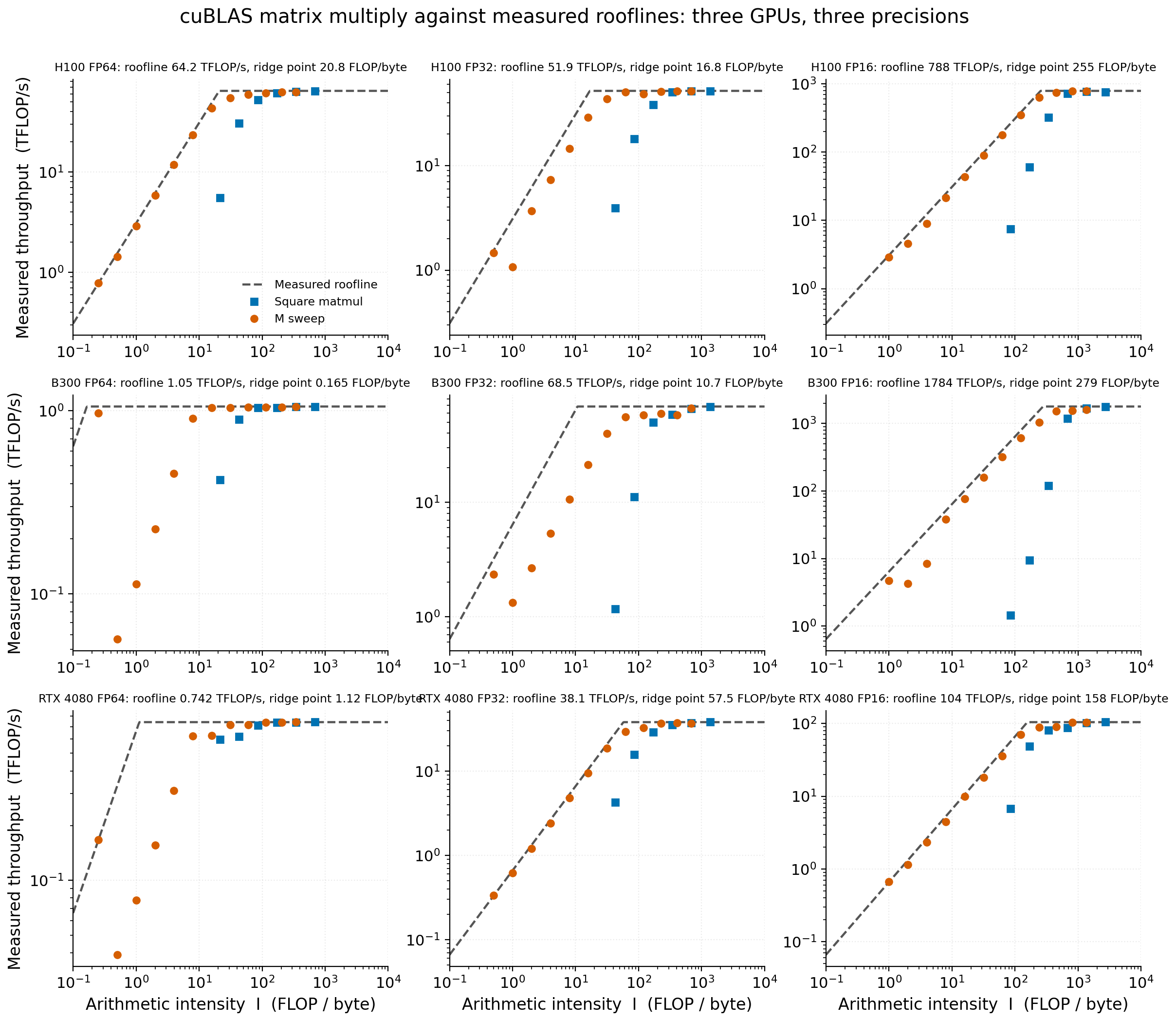

- Each precision stays at its own flat part. On H100, FP64 points level off at 64 TFLOP/s and FP32 points at 52 TFLOP/s, the flat parts of these two paths in Table 4.
- B300 FP64 points are all on the flat part. Its ridge point is 0.16 FLOP/byte, and \(M = 1\) gives \(I = 0.25\) FLOP/byte.
- Lower precision puts points farther right. Within a row, the same \(M\) gives \(I = 2M/\text{sizeof}\), larger for smaller sizeof.
M sweep
The M sweep fixes \(N = K = 8192\) and varies only \(M\): the weights of one linear layer stay the same while the number of tokens fed in at once grows from 1 to 8192. The same kind of matrix multiply then moves from \(I \approx 1\) FLOP/byte to several thousand, from the slope of the roofline to the flat part.
Figure 5 plots the FP16 M sweep of eight GPUs on its own, with \(M\) on the x-axis: the number of rows of \(X\) in \(X_{M\times K} \cdot A_{K\times N}\), which for an LLM linear layer is the number of tokens fed in at once. While \(M\) is small, FP16 has \(I \approx M\), so the x-axis reads about the same as \(M\) or as \(I\).
Each GPU’s ridge point is also converted to \(M\) and given in the legend: below that \(M\) a point lies under the slope, above it under the flat part.
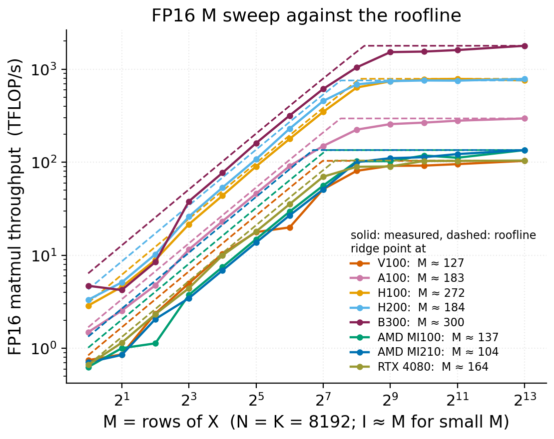
| \(M\) | \(I\) FLOP/byte | Throughput TFLOP/s | Bandwidth reached \(Q/T\) GB/s |
|---|---|---|---|
| 1 | 1 | 2.9 | 2875 (93% of \(B\)) |
| 16 | 16 | 43.7 | 2744 |
| 256 | 241 | 635 | 2637 |
| 2048 | 1365 | 788 | 577 |
Table 6: Four H100 points from Figure 5.
- The curve turns flat at the ridge point. In terms of \(I\), H100 turns flat at its ridge point of 255 FLOP/byte (\(M \approx 272\)). For larger \(M\), \(I\) falls below \(M\), since \(M\) is no longer much smaller than \(K\) and \(N\).
- On the slope, a few more rows cost no time. Throughput grows in proportion to \(M\) because the time barely changes: each call reads the whole 8192×8192 \(A\) (128 MiB in FP16). On the slope, the bytes of \(A\) read set the time, and a few more rows take no extra time.
- The bandwidth reached shows where the time goes. The formula’s \(Q\) divided by the time stays close to \(B\) on the slope, so the time goes to moving data; at \(M = 2048\), on the flat part, arithmetic sets the time and the bandwidth reached falls to 577 GB/s.
Points far from the roofline
Figures 4 and 5 also contain points far from the roofline. The roofline is an upper bound; how far below it a kernel falls depends on its implementation. There are four main cases:
- Small square matrices: launch overhead. On H100, FP16 square matrices with \(n = 256\) and \(n = 512\) both take 4.5 µs: the work differs 8-fold and the time is equal, so the time is almost all launch overhead (Section 4). Many small matrix multiplies put into one kernel (cuBLAS’s batched interface) pay this cost once.
- Small \(M\): the kernel cuBLAS selects. H100 FP16 takes 0.060 ms at \(M = 4\), longer than 0.050 ms at \(M = 8\). cuBLAS picks kernels by \(M\): \(M = 1\) is a GEMV with its own kernel, and the general kernel picked for \(M = 2\) and 4 is less efficient. B300 FP16 behaves the same at \(M = 2\) and 4. On these two GPUs, padding \(M = 2\) or 4 to 8 is faster, over twice as fast on B300 (0.064 → 0.028 ms).
- The same kind of effect appears near the flat part. RTX 4080 FP16 stays at 90 TFLOP/s from \(M = 256\) to 512 and reaches 103 at \(M = 1024\).
- The small-\(M\) points of FP32 and FP64 are much lower, and their time is constant over a range of \(M\). The cause differs; Section 7 covers it.
6. LLM inference: prefill and decode
The arithmetic and weight reads of LLM inference (using a trained model to generate text from an input) are mostly in the linear layers. By Section 2, a linear layer’s \(I\) is set by \(M\), the number of tokens fed in at once. Inference has two phases:
- prefill: the whole input at once. The input prompt (the input text) is computed in one pass, and \(M\) is the batch (the number of requests processed together) times the prompt’s token count. Once \(M\) reaches a few hundred, \(I\) exceeds H100’s \(I^*\), so prefill is compute-bound when the input is long.
- decode: 1 new token per step. Token \(t+1\) is generated from token \(t\), known only after the previous step finishes, so each step feeds in 1 new token per request; the intermediate results of earlier tokens (KV cache) are stored and not recomputed. \(M\) equals the batch, and at batch = 1, \(I \approx 1\) FLOP/byte, so decode is memory-bound.
The seven linear layers in one layer
A concrete model shows where the two phases fall. The model is Qwen2.5-7B (nominally 7 billion parameters, about 7.6 billion in fact), with 28 identical layers; layer 14, the middle one, is used here. It has seven linear layers, each with a different \(N\): q, k, v and o in the attention part, and gate, up and down in the MLP part.
Nsight Compute (NVIDIA’s kernel profiler, which reads hardware counters) measures these seven kernels on H100, H200 and RTX 4080. The x-axis is \(2MNK\) divided by the GPU memory bytes the counters record, i.e. \(I\) from the actual traffic; the y-axis is \(2MNK\) divided by the kernel time.
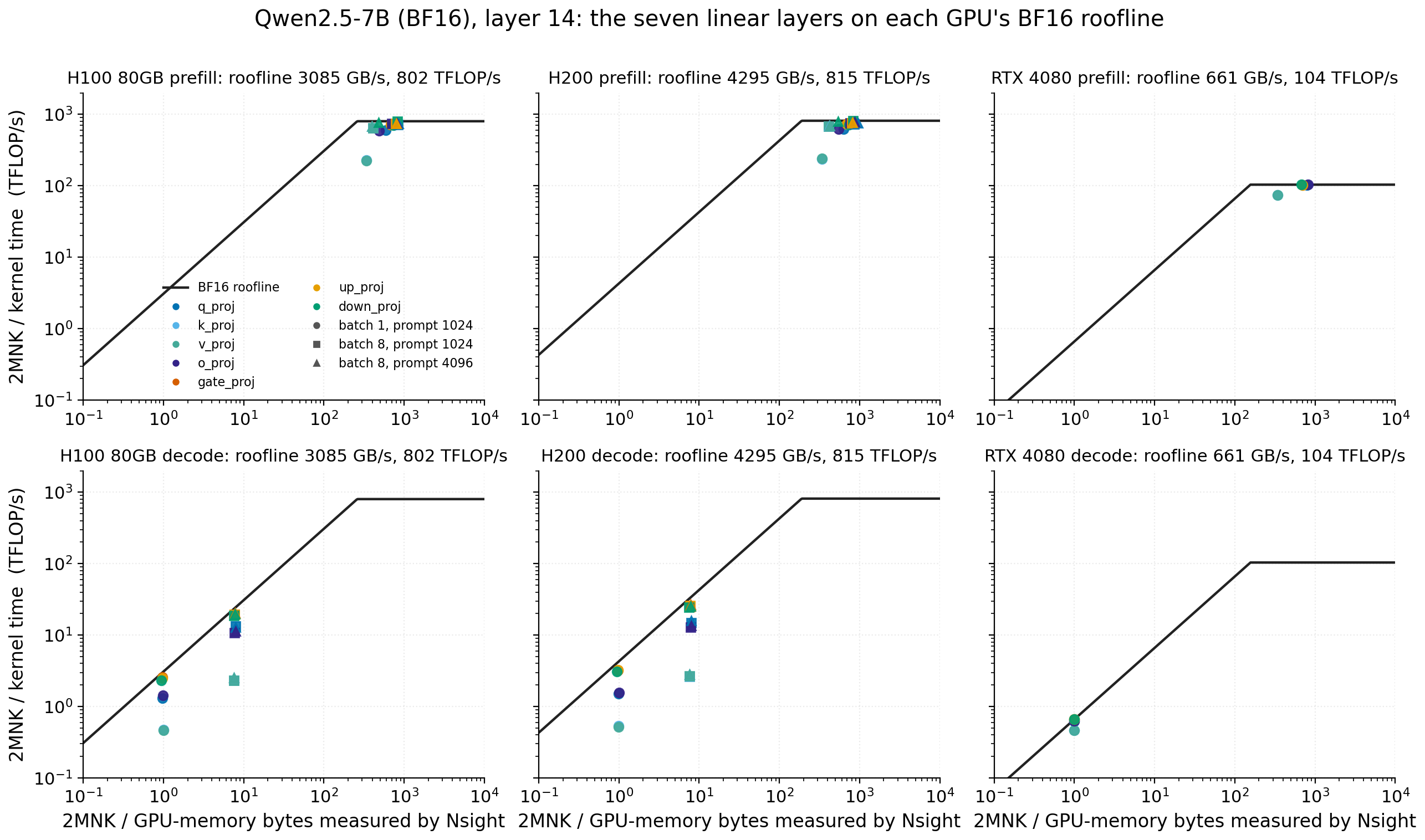
- prefill is close to the flat part. On H100, \(I\) is 340 to 850 FLOP/byte, all above the BF16 \(I^* = 260\) FLOP/byte. Except k and v at batch 1, throughput is 588 to 794 TFLOP/s, close to the flat part at 802. BF16 \(F\) is measured separately: 802 TFLOP/s on H100 and 815 TFLOP/s on H200, versus 788 and 756 TFLOP/s in FP16.
- decode is close to the slope. \(I \approx 1\) FLOP/byte at batch 1 and \(I \approx 8\) FLOP/byte at batch 8, as computed in Section 2. On H100, the three largest matrices, gate, up and down, reach over 80% of the slope and q and o about half; on RTX 4080, all but k and v reach over 93%.
- k and v are farthest from the roofline. Their output dimension is 512 (3584 for q and o), the smallest of the seven, so launch overhead takes the largest share.
Lower bound on time per decode step
One decode step is a chain of kernels. Each takes at least its own \(Q/B\), so a step takes at least its total bytes moved divided by \(B\). When the prompt is not long, other reads and writes are small and the largest item is the weights, which every step reads in full:
\[T_\text{decode} \ge \frac{Q_\text{weights}}{B}\]Here \(Q_\text{weights} = 15.23 - 1.09 = 14.14\) GB. 15.23 GB is all Qwen2.5-7B parameters in BF16; 1.09 GB of that is the input embedding table (a lookup table mapping token IDs to vectors), of which each step reads one row, so it is left out.
The decode times below come from running the model step by step in Hugging Face Transformers (a widely used inference library) with a 128-token prompt; the CPU issues each kernel one by one, with no inference framework such as vLLM.
| GPU | \(B\) GB/s | Bound ms | Measured ms | Bound ÷ measured |
|---|---|---|---|---|
| RTX 4080 | 661 | 21.4 | 24.3 | 88% |
| H100 80GB | 3085 | 4.58 | 11.56 | 40% |
| H200 | 4295 | 3.29 | 11.86 | 28% |
Table 7: Bandwidth bound and measured time per decode step at batch = 1.
Compute utilization at batch = 1
At batch = 1, the work per step is small. Excluding the embedding, there are 14.14 GB ÷ 2 bytes = 7.07 billion weights, each doing one multiply-add, so \(W \approx 14.1\) billion FLOP. On H100, \(W/F\) is 0.018 ms, less than 1/250 of the 4.58 ms bandwidth bound. Each weight read is used for one multiply-add, and less than 1% of H100’s compute is used.
The formula shows how to change this. At batch \(b\), each step feeds in \(b\) tokens and \(M = b\): the weights are still read once per step, so \(Q\) barely changes, while \(W\) grows \(b\)-fold and \(I \approx b\). While \(I\) is left of the ridge point, reading the weights still sets the time, and the extra tokens take almost no extra time: this is Section 5’s “a few more rows take no extra time” on the slope.
Counting the weights alone, H100 BF16 has \(I^* = 260\) FLOP/byte, so this holds until the batch reaches over two hundred. Each request’s KV cache is also read once per step and can no longer be ignored once the batch and prompt are large.
The measurements agree. In the bottom row of Figure 6, as the batch goes from 1 to 8, the decode points move along the slope from \(I \approx 1\) to \(I \approx 8\) FLOP/byte and throughput rises. Figure 7 shows the time per step against batch.
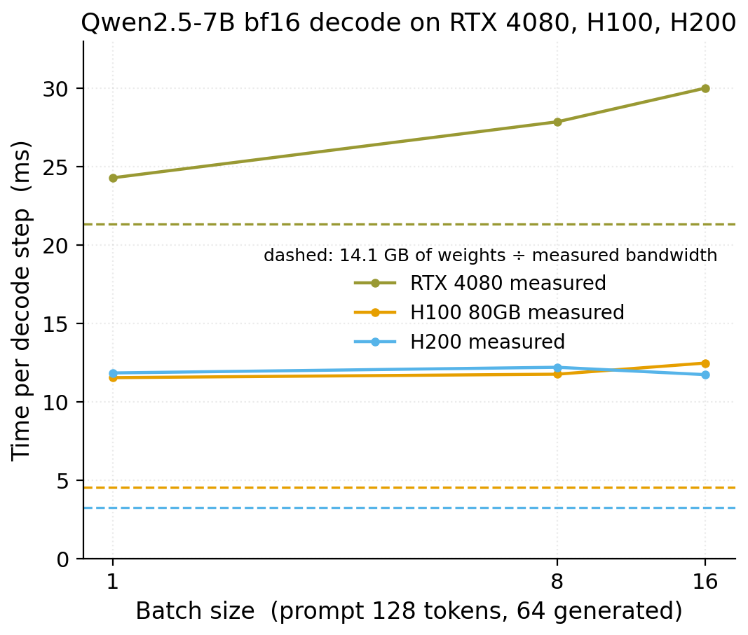
From batch 1 to 16, each step generates 15 more tokens, while the time per step rises 8% on H100 (11.56 → 12.50 ms) and 24% on RTX 4080 (24.3 → 30.0 ms); the time per token drops by an order of magnitude on both. This post does not break RTX 4080’s extra 24% down by kernel; H200 at batch 16 is slightly faster than at batch 1, within measurement noise.
This gain shrinks as the prompt grows. On H100, from batch 1 to 16, the time per step rises 93% with a 1024-token prompt (11.49 → 22.14 ms) and 4.4-fold with a 4096-token prompt (12.55 → 54.81 ms); per token, it falls to 1/8 and 1/3.7 respectively. Each request’s KV cache is read every step, and its size is proportional to the batch times the prompt length, so with long prompts it can no longer be ignored.
Measured time above the bound
In Table 7, RTX 4080 is near its bound, with weight reads taking 88% of each step; H100 and H200 measure 2.5 to 3.6 times their bound. If the extra time also went to moving data, H200, with 39% more bandwidth, would be faster; the two measure almost the same (11.56 vs 11.86 ms). So the extra time is spent outside data movement.
The most likely cause is how fast the CPU issues kernels. A step issues over a thousand kernels (28 layers, about 44 each), and each issue takes CPU time. On H100 and H200, many kernels finish before the CPU can issue the next, so the GPU waits idle; on RTX 4080, reading the weights is slow, the CPU has time to issue later kernels early, and the GPU waits less.
Inference frameworks such as vLLM use CUDA Graphs to submit a step’s kernels at once, to remove this cost. Where H100’s extra 7 ms or so and H200’s 8.6 ms go can be confirmed from the gaps between kernels in a profiler.
7. Where the model applies
The model has three limits, each with an example in the data:
| Limit | Example in the data |
|---|---|
| The roofline’s \(B\) is memory bandwidth; when data is read from L2, points can be above the roofline | RTX 4080 FP8 points are nearly twice the roofline (Figure 8) |
| The executed work can exceed \(2MNK\) | RTX 4080 FP64 takes 6.89 ms for every \(M\) from 2 to 32 (Figure 9) |
| Roofline applies to a single kernel | Each decode step takes 3 to 9 ms longer than the bandwidth bound (Section 6) |
Table 8: Three limits of the model.
Data read from L2
In the FP8 (1 byte per element) M sweep on RTX 4080, throughput for \(M = 16\) to 64 is 1.8 to 2 times the roofline. With the formula’s \(Q\), the bandwidth is 1200 to 1300 GB/s, close to twice the memory bandwidth, possible only if part of the data comes straight from L2: in FP8, \(A\) is 64 MiB, the size of L2, and stays in L2 across back-to-back runs.
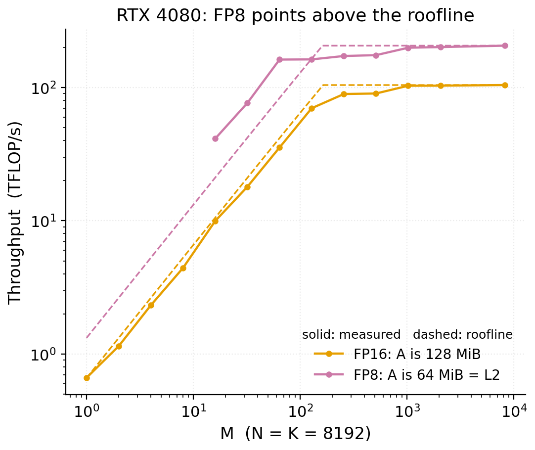
When the working set fits in L2, the real memory traffic is less than the formula’s \(Q\), and points plotted with that \(Q\) can be above the roofline. Then \(I\) should be recomputed from the real memory traffic measured by a profiler.
More operations executed than useful operations
RTX 4080 FP64 takes 6.89 ms for every \(M\) from 2 to 32, and B300 FP32 takes 0.20 ms over the same range. cuBLAS kernels split the matrix into blocks of a fixed number of rows and compute a full block even when \(M\) is smaller; this is padding. At \(M = 1\) a GEMV kernel is used instead and is unaffected.
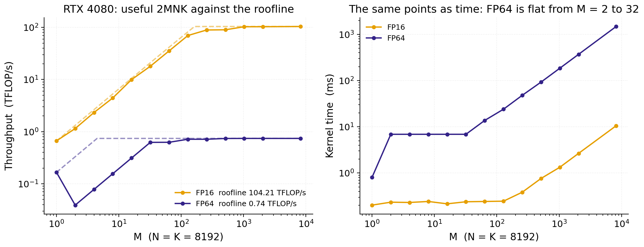
At \(M = 2\), RTX 4080’s FP64 kernel computes 32 rows, 2 useful, so useful throughput is 1/16 of executed throughput. FP16 padded to 32 rows would have \(I \approx 32\) FLOP/byte, still left of RTX 4080’s ridge point of 158 FLOP/byte; reading \(A\) sets its time, and the extra rows take no time. FP64’s ridge point there is 1.12 FLOP/byte, so padding’s extra operations set its time directly. So padding slows a kernel only when the padded \(I\) exceeds the ridge point.
Time outside a single kernel
Roofline is a model of a single kernel. A program consists of many kernels, and besides the kernels’ own time it also spends time outside them (overhead): running the Python interpreter and framework code, issuing each kernel from the CPU, and synchronizing the CPU and the GPU.
Frameworks such as PyTorch run asynchronously: while the GPU runs one kernel, the CPU is already issuing the next ones. When kernels are large, the GPU’s execution time hides this overhead; when kernels are small and numerous, the GPU finishes them faster than the CPU issues them, sits idle waiting, and the CPU side sets the program’s time. The time each decode step in Section 6 takes beyond its bandwidth bound includes both kernels falling short of their roofline and overhead outside the kernels; how much each contributes can only be told from a profiler’s kernel timeline.
8. Summary
- A kernel takes at least \(\max(W/F,\ Q/B)\). Comparing \(W/Q\) with \(F/B\) shows whether bandwidth or compute limits it.
- \(W/Q\) depends on the operation’s shape and precision and can be computed directly from the formula; \(F/B\) must be taken for the compute path the kernel actually uses, and on H100 ranges from 10.7 to 255.
- For a kernel limited by bandwidth, reduce bytes moved and raise \(I\); for one limited by compute, move to a higher flat part, such as Tensor Cores or lower precision.
- When a measured point is far from the roofline, the cause lies outside the model: launch overhead, the kernel cuBLAS selects, padding, or idle waits between kernels.
- In LLM inference, prefill lies under the flat part and decode under the slope. Each decode step reads the weights at least once, and the larger the batch, the more tokens share this read.
All data tables, benchmark sources, plotting scripts and the decode timing script are in the companion repository.